Second Submission to the Senate Inquiry into Wind Turbines

Second Submission to the

Senate Inquiry into Wind Turbines

Peter Bobroff, AM

Introduction

I lodged one submission before the initial deadline where I addressed wind related issues for which I already had analysed data. Subsequent communication from the Committee staff raised further areas of interest. Those within my area of interest were:

Capital and operating costs of wind
Actual power delivery by wind farms
Times at which wind power was delivered
Projected impacts on global temperatures

This second submission addresses these issues. I don’t suggest that I can provide definitive answers to all of these complex questions, but I hope to broaden the readers’ understanding.

1. Capital and operating costs of wind and comparison to conventional power generation
1.1. Short Run Marginal Cost
1.1.1. Fuel Cost
1.1.2. Thermal Efficiency
1.1.3. Variable Operating and Maintenance Cost
1.1.4. Renewable Energy Certificate
1.1.5. Final Short Run Marginal Cost
1.2. Long Run Marginal Cost
1.2.1. Interest Costs
1.2.2. Fixed Operating and Maintenance Costs
1.2.3. Final Long Run Marginal Costs
1.3. Profitability under different marginal costs
1.3.1. Long Run Profitability
1.3.2. Short Run Profitability
1.3.3. Short Run Profitability without RECs
1.3.4. Long Run Profitability without RECs
1.4. Summary – Capital and operating costs of wind
2. Actual power delivery by wind farms 2014
2.1. Plots
2.2. Histograms
2.3. Tabular
2.4. Summary – Actual power delivery by wind farms
3. Times at which wind power was delivered
3.1. MACARTH1 on 2014-09-17 one generator for one day
3.2. MACARTH1 during 2014-09 one generator for one month
3.3. All wind farms on 2014-09-17
3.4. All wind farms during the month of 2014-09 by unit
3.5. All wind farms during the month of 2014-09 by date
3.6. All wind farms during the month of 2014-03 by unit
3.7. All wind farms during the year 2014 by unit
3.8. All wind farms during the year 2014 by month
3.9. Summary – Times at which wind power was delivered
4. Projected impacts on global temperatures
4.1. Impact of renewables on atmospheric CO2
4.1.1. The Pessimistic Scenario
4.1.2. The Optimistic Scenario
4.2. Impact of CO2 concentrations on global temperatures.
4.2.1. MAGICC outputs
4.3. Summary – Projected impacts on global temperatures
5. Conclusions

1 Capital and operating costs of wind and comparison to conventional power generation

The actual costs are almost certainly Commercial in Confidence.

The Australian Energy Market Operator (AEMO) publishes generic generator parameters which can be combined with actual generator dispatch data and actual state price data to allow estimated Marginal Costs to compared with actual Prices.

AEMO publishes multiple sources of these generic generator parameters which do not always agree. Parameters are missing for some generators that dispatched power in 2014. AEMO does not assign unique generator and station identifiers so the matching of data between AEMO spreadsheets often requires considerable effort and cannot be relied upon to be 100% accurate.

In this discussion of capital and operating costs, only generators dispatching more than 40,000 MWh in 2014 have been considered. The 40 generators dispatching less than 40,000 MWh in 2014 have very high marginal costs for Interest on capital and Fixed Operating and Maintenance and this results in poor plot scales for viewing the larger more important generators.

1.1 Short Run Marginal Cost

This is the extra cost of generating an additional 1MWh of electricity. It neglects all annual costs such as: Interest on capital and operating/maintenance costs.

SRMC ($/MWh) is defined a:

Thermal Efficiency (GJ/MWh) x Fuel Cost ($/GJ)
+ Variable Operating and Maintenance cost ($/MWh)
– Renewable Energy Certificate value (-$35.24 for renewables, +$3.52 on fossil fuels)

1.1.1 Fuel Cost

The Fuel Costs were derived from the type of fuel and the geographic zone of the generator.

Wind and Hydro have zero fuel costs but there could be a monetary value assigned to the release of dam water for generation in competition to release for irrigation.

Gas is usually much more expensive than Coal.

These scatter plots show a point for each generator at the year of commissioning. The dot size represents the size of the generator in MW.

1.1.2 Thermal Efficiency

This relates the theoretical heat energy of the fuel in GJ to the electrical energy produced from the fuel in MWh.

AEMO parameters give Hydro about 82% efficiency. Presumably that is the conversion of gravitational potential energy into electrical energy. The figure is unimportant as the Hydro fuel cost is assumed to be zero.

AEMO parameters give Wind 100% efficiency. It is unlikely that the kinetic energy of the wind in the blade circle is converted to electrical energy with anything like 100% efficiency but it is unimportant as the fuel cost is assumed to be zero.

The increasing efficiency of modern gas turbines is evident.

1.1.3 Variable Operating and Maintenance Cost

These costs are related to the amount of power being generated. Open the throttle and the VOM costs go up.

Coal plants and some gas turbines have extremely low VOM costs, even lower than wind apparently.

1.1.4 Renewable Energy Certificate

Wind generators receive one REC for each MWh they generate. RECs can be traded on a market with average price in 2014 being about $35. Electricity retailers had to source about 10% of their energy from wind. This seems to equate to a 10% rise in the effective price of non-wind energy for the retailer.

1.1.5 Final – Short Run Marginal Cost

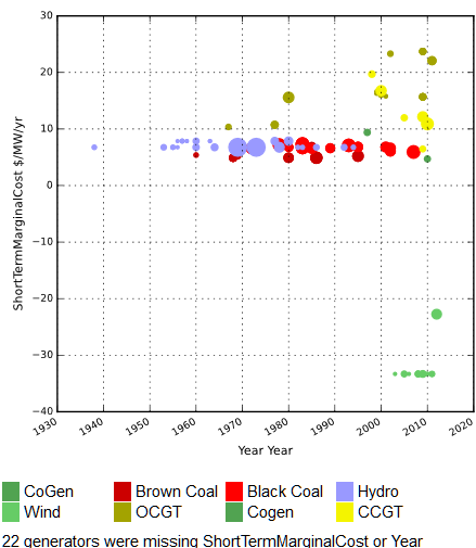This is the total of: Fuel Cost by Thermal Efficiency, VOM costs and the REC.

The Combined Cycle Gas Turbines appear to be steadily improving their SRMC. Coal and Hydro tend to be much lower than Gas.

The negative SRMC of Wind is due to the $35/MWh Renewable Energy Certificate.

1.2 Long Run Marginal Cost

This adds the annual costs of Interest on Capital and Fixed O&M costs to the Short Run Marginal Cost. To avoid bankruptcy, a company must sell its product for at least the LRMC.

LRMC ($/MWh) is defined as:

+ Short Run Marginal Cost ($/MWh
+Interest at 10% on Capital and Capital Works / Energy dispatched in 2014 (MWh)
+Fixed Operating and Maintenance cost ( $/MW/year) / Energy dispatched in 2014 (MWh)

1.2.1 Interest Costs

No capital cost parameters were available for Hydro, so zero has been assumed. Perhaps all the debt has been repaid?

The 10% pa capital cost came from What is Normal Profit for power generation? Simhauser and Ariyaratnam p14 and covers debt or equity finance.

The annual interest cost has been reduced to a marginal cost by spreading it over the energy generated in 2014.

Marginal interest costs for Wind appear greater than those for Coal and some Gas

1.2.2 Fixed Operating and Maintenance Costs

Hydro generators have quite a spread of FOM Costs, probably reflecting different amounts of energy generated in 2014.

Wind has higher FOM Costs than Coal and most of the CCGT.

1.2.3 Final – Long Run Marginal Costs

Hydro LRMC is very low, due mostly to the assumed lack of Interest on Capital. This might not be correct, but no data could be found.

Most Coal, Wind and CCGT gas fall in the range 30-70 $/MWh.

Open Cycle Gas Turbines are often much higher.

1.3 Profitability under different marginal costs

Long Run Marginal Cost
Short Run Marginal Cost
Long Run Marginal Cost with no Renewable Energy Certificates
Short Run Marginal Cost with no Renewable Energy Certificates

All of these are covered by showing:

the Regional Reference Prices (state wholesale spot price) as a histogram of occurrence against Price in $/MWh. Separated by state.
the Marginal Costs as a bar chart of Registered Capacity in MW against cost in $/MWh. Separated by generator type

The X axes are identical to facilitate comparison.

1.3.1 Long Run Profitability

If a company cannot consistently sell its generated power at above its Long Run Margin Cost, it will eventually go bankrupt.

If AEMO’s generic parameters are approximately correct, most generators are unprofitable, except for Hydro where Interest costs have been assumed to be zero.

Why do the generation companies persist? Things are obviously not as simple as they seemed at first sight.

1.3.2 Short Run Profitability

The wholesale electricity market is a short term spot market. The lowest bids are accepted. If you can’t win contracts at your Long Run Marginal Cost you will go broke but if you can win bids at above your Short Run Marginal Cost you will go broke more slowly.

Most Short Run Marginal Costs are below the state wholesale prices so there is much scope for this short term death spiral.

This is known as the Missing Money Problem. The suggestion that infrequent price spikes allow some recompense seems inadequate.

The REC gives Wind a particular advantage in being to able to drive prices into the negative. This does occur.

1.3.3 Short Run Profitability without RECs

Removing the RECs would lessen the ability of wind generators to drive the price into the negative region but do nothing to solve the Missing Money Problem and to restore the industry to long term profitability.

1.3.4 Long Run Profitability without RECs

The main effect of withdrawing RECs is to make most Wind generators very unprofitable in the Long Run.

1.4 Summary – Capital and operating costs of wind

Given the assumptions stated earlier and the incompleteness of data, these observations are offered:

The spread of wholesale prices is usually less than the Long Run Marginal Costs of most generators. Money is being steadily lost.
The Short Run Marginal Cost of most generators is below the spread of wholesale prices. Understandably, generators are using this and bidding low to go broke as slowly as possible.
Without the Renewable Energy Certificates, the Long Run Marginal Cost of Wind is far more than that of fossil fuels.
Renewable Energy Certificates allow wind generators to bid negative prices and still exceed their Short Run Marginal Cost.

The national electricity market does not seem to be developing sustainable prices.

2 Actual power delivery by wind farms – 2014

The following plots and histograms are based on AEMO 5 minute data for every generator attached to the grid for the whole of 2014 – about 20 million samples.

2.1 Plots

Over the whole of 2014, Wind provided 4% of the energy to the grid. Coal provided 75%.

The daily plots show Coal averaging more than 15GW on most days with Wind averaging less than 2GW on most days.

There is a small change throughout the year.

2.2 Histograms

We are now interested in the amount of power generated, irrespective of the time of day, day of month or month of the year and irrespective of which unit generated it. These histograms show what proportion of the time a certain power level was generated. In the first (Coal), the maximum of about 17GW was being generated almost 16% of the time. 20GW was generated only about 1% of the time

Coal is dominant, delivering between 11GW and 21GW when the demand required it. There is no need to look at daily or monthly data as power is generated when required.

Gas provided about 1GW to 8GW of peaking power whenever it was required. There is no need to look at daily or monthly data as power is generated when required.

Hydro provided about 400MW to 5GW of power whenever it was required. There is no need to look at daily or monthly data as power is generated when required.

Wind provided from a tiny 5MW to nearly 3GW controlled by the vagaries of the wind.

Wind is of significance only in South Australia which has little coal and must use gas whose fuel price is increasing.

2.3 Tabular

Here are the statistics as numbers.

2.4 Summary – Actual power delivery by wind farms

Wind is unreliable and other generators need to be online ready for it to fail.

From AEMO spreadsheet, contribution factors specify the portion of installed capacity expected to be available to meet peak demand. The AEMO table has been pruned of some rows and the X for 100% column derived.

The table shows, that to meet an expected peak load of 1GW, 45GW of wind should be installed in NSW and Qld. South Australia could get by with installing 12GW for each 1GW of expected demand.

Without the subsidy of Renewable Energy Certificates, Wind’s Long Run Marginal Cost is already twice that of Coal. If NSW and QLD need to install 45 times the required capacity, then it becomes 90 times more expensive.

The proposal to replace Coal by Wind in the major states is absurd.

3 Times at which wind power was delivered

AEMO provides data covering the power dispatched by almost all generators connected to the grid for every 5 minute period. Data is available for over 30 wind farms. This analysis has been restricted to 2014, but still contains over 3 million data points for wind alone.

It is easy to lose track of the fine detail when attempting to comprehend this amount of data, so we will start simply and then expand the view out and up.

The Times at which can be interpreted as:

the hours of day – variations throughout the day
the days of the month – variations between days
the months of the year – variations between the seasons

When looking at one wind farm, MACARTH1 will be used as it is the biggest at 420MW.

Most of the following plots will be in terms of the Capacity Factor of the generator which is the actual power dispatched to the grid expressed as a percentage of the Registered Capacity (maximum). This facilitates the comparison of generators of different size.

3.1 MACARTH1 on 2014-09-17 – one generator for one day

When looking at one generator for one day, a simple line plot clearly shows each 5 minute period with no statistics needed.

The great variation in output from one wind farm during the day is obvious.

3.2 MACARTH1 during 2014-09 – one generator for one month

Now we have expanded to all the days in the month of September 2014. All 5 minute points are still visible but now encoded by colour. Colour is not as clear as the plot line in the previous plot, but the minute to minute variation can still be seen.

The date shown earlier, 2014-09-17, can be seen as unexceptional. There are windier days and calmer days.

MACARTH1 reached 100% capacity on occasions.

There appear to be 3 or 4 calm days followed by a few windy days, probably corresponding to the passage of high pressure systems from west to east over Australia.

3.3 All wind farms on 2014-09-17

Here we have returned to 2014-09-17 but are now showing all wind farms. All 5 minute points are still visible.

Some generators reached 100% capacity briefly. Others never reached 50%.

MACARTH1 is not exceptional with other units doing better and others doing worse.

3.4 All wind farms during the month of 2014-09 by unit

For the first time, the basic 5 minute data points are no longer visible. Each point in time is now the average of such points for all days of the month. The day to day variation is now lost.

There appears to be a period of reduced wind around 9am and another around 7pm (19:00 hours), but this is a very weak observation.

At no time of day did any generators have monthly averages of over 50% capacity.

Most wind farms did better than MACARTH1 during September 2014.

3.5 All wind farms during the month of 2014-09 by date

Each point in time is now the average of such points for all generators on that day. The unit to unit variation is now lost.

In comparison with the previous plot, there is more variation from day to day than from generator to generator. Weather causes more variation than siting.

On some days wind gets up to 50-75% capacity for much of the day but on others is below 10% for much of the day.

3.6 All wind farms during the month of 2014-03 by unit

March 2014-03 was calmer than September 2014-09.

SNOWTWN1 (99MW) reached a monthly average of 54% capacity briefly between 8pm and 10pm but most generators did far worse at most times.

3.7 All wind farms during the year 2014 by unit

SNOWTWN1 (99MW) reached a yearly average of almost 50% capacity briefly between 9pm and 10pm but most generators did far worse at most times of the day.

There is some suggestion of wind changes at about 9am and 7pm (19:00 hours).

3.8 All wind farms during 2014 by month

Here each cell represents the average of all wind generators and the average of all days in the month. This process has suppressed all the variation between generators and the variation between days.

2014-03 March is the worst month and 2014-07 July was the best month.

3.9 Summary – Times at which wind power was delivered

The above plots demonstrate:

the output of a single wind farm can vary widely during a day , from very little to 100% capacity.
a single wind farm almost never produces 100% capacity all day
the output of a single wind farm can vary widely from day to day
the total output of all wind farms varies during a day, but much less than the variation of single wind farms
the total output of all wind farms varies from day to day, approximately between 10% to 75%
the total output of all wind farms varies throughout the months, from about 20% to 45%

There is almost no storage on the grid. Energy must be generated to meet the instantaneous demand. The minute to minute wind variations must be countered by matching variations on other generators which can no longer run at steady efficient settings. Other generators must be kept on standby in case of a rapid decline in wind. This is expensive and wasteful.

Wind without storage does not replace any other generators.

4 Projected impacts on global temperatures

This can be approached in 2 steps:

the projected impact of renewables on atmospheric CO2 concentrations
the projected impact of CO2 concentrations on global temperatures.

4.1 Impact of renewables on atmospheric CO2

There has been a massive growth in wind capacity since 1996 and in solar capacity since 2006. The claimed reductions in tonnes of CO2 emitted are very large.

However there has been no detectable change in atmospheric CO2 trends over this time period. The trend remains at slightly less than 2 parts per million increase per year, so:

Either some unknown natural process has commenced and is cancelling the savings
or the CO2 concentration savings from current levels of renewables are non-existent.

4.1.1 The Pessimistic Scenario India, China, Japan, Germany and Russia are all building more coal-fired generators so a pessimist might suggest that the CO2 concentration trend might increase from 2 to 3 ppm per year. The 2050 concentration would then be 505 ppm.

4.1.2 The Optimistic Scenario The EU (and UK in particular) plans to increase renewable generators, so an optimist might suggest that the CO2 concentration trend might decrease from 2 to 1 ppm per year. The 2050 concentration would then be 435 ppm.

4.2 Impact of CO2 concentrations on global temperatures.

MAGICC is a Model for the Assessment of Greenhouse-gas Induced Climate Change. It is a set of coupled gas-cycle, climate and ice-melt models that allow the user to determine the global-mean temperature of user-specified greenhouse gas emissions. It was developed by the US based National Center for Atmospheric Research and represents the view of the IPCC Fourth Assessment Report.

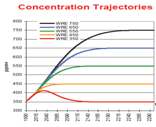The Pessimistic Scenario is the Reference Scenario in MAGICC and WRE750 has been chosen to give about 500 ppm in 2050. The Optimistic Scenario is the Policy Scenario in MAGICC and WRE450 has been chosen to give about 435 ppm in 2050.

The User Model was used with default values except that Climate Sensitivity was set to the AR4 most likely value of 3°C for a doubling of CO2. The time period selected was 2015-2050.

4.2.1 MAGICC Outputs

4.3 Summary – Projected impacts on global temperatures

The difference between the Optimistic and Pessimistic Scenarios at 2050 is the benefit from the world renewables policy and is about 0.25°C. The cost of the the world renewables policy is hundreds of billions of dollars.

There have recently been several papers suggesting that the Climate Sensitivity may be lower than 3ºC. Some are suggesting as low as 1.5ºC. This would reduce the benefit to about 0.12ºC.

5 Conclusions

When ample coal is available at current prices, wind is too expensive and unreliable to supply the grid.
The fashionable proposal to completely replace Coal in the 3 major states by Wind is absurd.
If ample coal is not available (South Australia) and gas prices rise, wind might cost effectively reduce gas consumption. An alternative would be the building interconnectors to access more distant coal generators as has been done for Tasmania under Bass Strait.
All the world’s current wind capacity has had no effect on CO2 concentrations and so can not have had any effect on temperature.
MAGICC outputs shows that a massive world-wide effort to increase wind capacity might save 0.25ºC by 2050. A proportional Australian effort would have contributed virtually nothing.